Welcome to the next level in our learning series. The subject is Programming With Basic Ladder Diagram The prerequisite for this material is our previous part in the learning series, PLC Part 2 Intro To CODESYS. Something else that may help, take a look at the setup for a DIY PLC Training station. The exercises for this series are designed to work with the training station described but you can cover a lot of the material using the CODESYS built in simulator if you chose.

To get an idea what’s covered here, take a peek at the table of contents. You’ll see that the focus is on learning how to program with Ladder Diagram language. At the end of part 3 you will be writing and testing programs made up with common instructions like Contact, Negated Contact, Coil, Set Coil and Reset Coil.
Table of Contents
Basics Of Ladder Logic
Ladder Elements In Basic Ladder Diagram
The Ladder Diagram (LD) programming language is made up of ladder diagram elements. These elements are:
- Networks (sometimes called rungs), visible as horizontal lines in the editor.
- Instructions, different instructions appear as different symbols or blocks.
- Branches, made up of vertical and horizontal lines branching off of networks.

Networks are scanned 1 line at a time, from top to bottom. It is like climbing down the rungs of a ladder. Instructions on the horizontal lines are processed in order from left to right, like reading a book.
A network with no instructions will show up as an empty space. Consider removing empty spaces if they appear to keep things cleaned up.

There are fundamentally two types of instructions, input and output. Instructions have variable names assigned. Variable names identify a piece of data. Variables do not necessarily have to be specific PLC addresses. Variables can be created (declared) and assigned to instructions when specific PLC addresses are not suitable. Instructions related to inputs monitor the data from the assigned variable and are placed to the left of a network. Instructions related to outputs control the data to the assigned variable and are placed on the right side of a network.

Ladder Diagram (LD) is a popular PLC programming language because it is designed to resemble ladder electrical drawings. Electricians and technicians are familiar with the concept of electrical continuity. That a circuit must have a path for current to complete the circuit in order to operate. A ladder electrical diagram shows switching devices to the left and load devices to the right.

To interpret the ladder diagram programming language (ladder logic) we need to grasp the concept of logical continuity. Where input instructions to the left of the network provide a path of TRUE conditions to the output instructions at the right.
Instructions For Basic Ladder Diagram: Contact, Negated Contact And Coil
The Contact is an input instruction. It is assigned a variable with BOOL (1 bit) data type. As an input type instruction it will monitor the bit of the assigned variable.
The instruction condition will be TRUE if the bit is TRUE ( ON, equals 1).
The instruction condition will be FALSE if the bit is FALSE (OFF, equals 0).

The Negated Contact is an input instruction. It is assigned a variable with BOOL (1 bit) data type. As an input type instruction it will monitor the bit of the assigned variable.
The instruction condition will be FALSE if the bit is TRUE ( ON, equals 1).
The instruction condition will be TRUE if the bit is FALSE (OFF, equals 0).
The result of the Negated Contact is the opposite of the Contact. That is why it is called Negated

The Coil is an output instruction. It is assigned a variable with BOOL (1 bit) data type. As an output instruction it will control the value of the assigned variable.
The instruction is TRUE if input conditions to the left provide a path of logical continuity. So long as the instruction is TRUE the bit will be TRUE ( ON, equals 1) for the assigned variable.
The instruction is FALSE if input conditions fail to provide a path of logical continuity. So long as the instruction is FALSE the bit will be FALSE (OFF, equals 0) for the assigned variable.
An important rule of thumb for the Coil instruction is that a Coil assigned a particular variable must be scanned only once per PLC scan cycle. If Coils are assigned the same variable in more than one location this increases the risk of multiple scans per cycle, making the behavior of the output erratic.

In the next few exercises, we will begin programming in the LD language. Starting with one simple network that we will test in simulation mode. Then we will build from there, step by step, to create a program to run on the training station. It will test our real world I/O to make sure the slave device is wired correctly.
Exercise 4 – Create A Simple Network With Basic Ladder Diagram
In this exercise we create a network that operates with one input connected to a pushbutton and one output connected to an LED. While we are doing that we will learn how to insert a new network, how to place Coils and Contacts on a network and how to assign addresses to the instructions.
For this exercise, our program plan is this:
- While PB1 is pressed the red LED will be on
The components chosen for the plan are PB1 and the red LED.

The plan has all the information we need to create the program except we need to know what the address is for each of the connected I/O components.
So, here is our plan once again, please check the diagram I/O Connections from the section PLC Part 2 Intro To CODESYS and find the addresses to complete the plan.
- While PB1 (at address______ ) is pressed the red LED (at address______ ) will be on.
To get ready for programming, we will save our project, “Training_Station_Base” from Exercise 3 with a new name. So, make sure you have saved a copy of “Training_Station_Base”.
With the project “Training_Station_Base” open, from the File menu select Save Project As.
Save with new name “Ladder IO Test”.

To open the editor, right click PLC_PRG from the devices view and select Edit Object. Alternately you can double click PLC_PRG.

Placing Instructions for Basic Ladder Diagram
When the ladder editor opens, the workspace will appear at the center of the screen. An empty network, numbered as #1, is in place ready for instructions to be added. If you click the mouse in the network area a yellow region appears with pink in the margin. This is the cursor, indicating the network is selected for editing.
The next step is to place a Contact instruction on the network. There are 4 easy ways to place instructions:
1 . Select instruction from the toolbar, if a network is selected for editing then available instructions will be blue. Greyed out instructions are not available. Click the network area and then click the desired instruction.


3 . Select from the FBD/LD/IL dropdown menu.

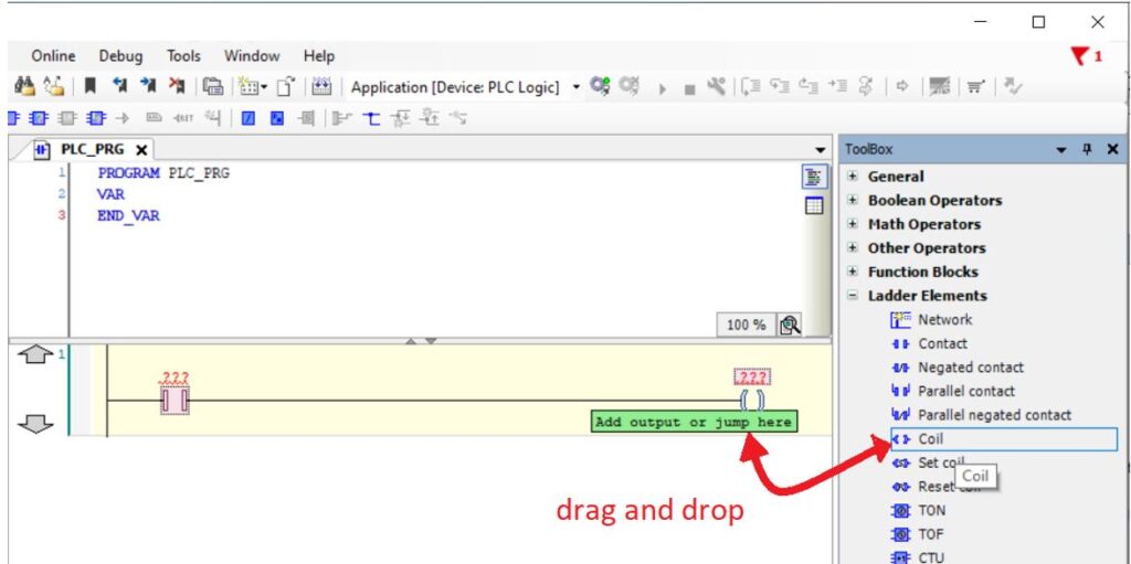
4 . Or, drag and drop from the toolbox, the toolbox is the window to the right with a list of instructions.

For this example, we will use the toolbox. Expand the heading Ladder Elements to show a list of basic instructions. Find the Contact instruction, click and hold to drag to the network area. A grey box will appear with the words “Start Here”. Bring the mouse cursor to the box until it turns green then release to drop the instruction.

The next step is to place a Coil instruction on the network. In similar fashion, drag and drop the Coil into place.
Assign Variables For Basic Ladder Diagram
To assign a variable to the Contact, click where you see the three question marks (???) then type in the address. This Contact is for the input connected to PB1. Think back to when you looked up the addresses for the I/O components. What is the address for PB1?

The Coil on this network is for the red LED. What is the address for the red LED? Assign the variable to the Coil.

Once the variables have been assigned, the network is complete. This is a good time to save the project.
This concludes Exercise 4
Exercise 5 – Simulation Of A Simple Network
In this exercise we will transfer our application to the simulation environment and run the program to see how the network works.
An online connection to a PLC is required to transfer files and to monitor the PLC status. In PLC jargon transferring files from the PC to the PLC is called downloading. Transferring files from the PLC to the PC is called uploading.
The steps for online connection and file transfer are mirrored in the simulation mode.
Enable Simulation
To start working with the simulation environment, from the Online menu select Simulation

Notice the red box in the status bar, a reminder that the simulation mode is active.

Login
The next step is to connect online with the PLC simulator. The online connection is established with the Login command. The Login and Logout commands are available from the Online menu. Alternately you can select Login or Logout from the toolbar.
Select Login.

When logging in, the application on the PC is compared to the simulator’s current application, if any. Based on that comparison you may be prompted by one of the following:
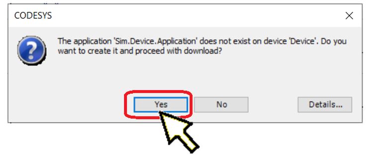
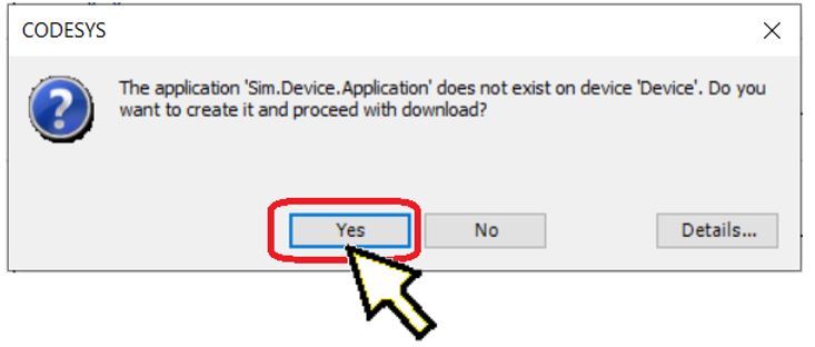
1 . A dialogue box indicating that no application exists. This happens if the simulator has no application currently loaded Connecting and downloading an application is our objective. So, the correct answer is Yes, to confirm the download.
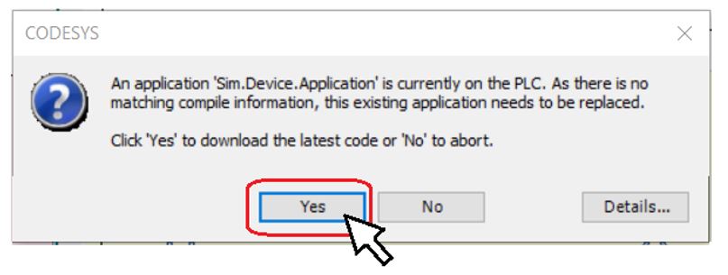
2 . A dialog box indicating an application is currently loaded but no matching compile information. This happens when the application loaded on the simulator is from a different project. Click Yes to confirm the download.
3 . A dialog box with 3 login options. This happens when the application on the PC is does not match the simulator’s current application and you must chose how to proceed.
a) Login with online change – Only loads the changed part of the application and does not require the application to stop to allow the change.
b) Login with download – Loads the complete application. Any running application would have to be stopped to accept the download. It may automatically restart or a manual restart may be necessary.
c) Login without any change – No changes will be loaded. The online connection will proceed but the application displayed on the PC will not match what is running on the simulator. This makes the view inaccurate while monitoring from the workspace.
Either of the first two options are acceptable for our purpose. It makes little difference in the simulation environment if we must restart the application. The third option, Login without any change, is not suitable since our objective is to download the application. Once a selection is made then click OK.

4 . A dialogue box indicating no online change is possible. This happens when the application on the PC is significantly different than simulator’s current application. Click Yes to confirm the download.

After logging in, notice the red box in the status bar. It is a reminder that the simulator needs to be started.

Running The Application
The Start and Stop commands are available from the Debug menu. Alternately there are Start and Stop buttons on the toolbar.
Select Start to run the simulator.

Notice the green box in the status bar, an indicator that the simulator is running.

When the development system is online our view will change from edit mode to monitor mode. When logging in you may have noticed a change to the display in the workspace. The vertical line, sometimes called the “rail” is highlighted blue. The horizontal line to the left of the Contact is highlighted blue as well. The blue line represents the path of logical continuity, the path of TRUE conditions that could enable an output if all conditions are satisfied.
The Contact is an input instruction. It is assigned a Boolean variable, the address %IX0.0. The value of the bit, at %IX0.0, is FALSE so the condition for the Contact instruction is FALSE. This is where the path of logical continuity ends and the Coil remains FALSE.

So how do we test the network in simulation mode, when we have no real input component to switch on or off? We need to set the value of the BOOL, at %IX0.0, to TRUE to complete the test.
This is the method. Double click on the Contact instruction. A blue box with the word “TRUE” appears. This is a preparation to write a value of TRUE to the simulator memory. Double click again and a black rectangle that says “FALSE” will appear in preparation to write the value of FALSE to the assigned variable. Each double click toggles the value back and forth. But the value is not actually written to memory until the next step.

To write any values that we wish to change, to memory, do the following. Place the mouse cursor anywhere in the workspace and right click. Then select Write All Values of Device.Application.

Use the method, just described to set the value of the Contact at %IX0.0 to TRUE. The Contact will now be highlighted blue, this indicates the condition for the instruction is TRUE. The vertical line to the Coil is blue and so is the Coil instruction. There is a path of logical continuity to the output instruction. The variable assigned to the Coil, %QX0.0 will be TRUE in memory.

Repeat the method to set the value of the Contact at %IX0.0 to FALSE. The network appears as it did before. The Coil at address %QX0.0 is FALSE once again.
We can summarize, So long as the Contact is TRUE the Coil is TRUE. The Contact is for PB1, the Coil is for the red LED. This satisfies our program plan, while PB1 is pressed the red LED will be on. Mission accomplished!
The method to write values is available for other instructions as well. Try double clicking the Coil instruction in preparation to write the value TRUE. Then go ahead, right click and select Write All Values of Device.Application.

What was the result? Did the Coil turn blue? If we have written a value of TRUE to the Coil, what could explain the result?
From the toolbar, find the Stop button ![]() and click to stop the application. Repeat the attempt to write the value TRUE to the Coil. What is the result?
and click to stop the application. Repeat the attempt to write the value TRUE to the Coil. What is the result?
From the toolbar, find the Start (Play) button ![]() and click to start. What now? What is the explanation for the behavior of the Coil?
and click to start. What now? What is the explanation for the behavior of the Coil?
The answer is related to the PLC Scan. When the application is running, it is repeatedly scanning the network every few milliseconds. At each scan it will recognize that the Contact instruction is FALSE, breaking the path of logical continuity and set the Coil instruction to FALSE. We may have written the value TRUE to the Coil but it would be set back to FALSE within one scan. If we stop the application, the network is not being scanned. We can write the value TRUE to the Coil and it will remain until the application is restarted.
When we have finished the simulation, stop the application, logout to disconnect and then turn off simulation mode from the Online menu.

This concludes Exercise 5.
Exercise 6 – Network With AND Relationship
In this exercise we will add to the existing program and create a network that operates with two pushbutton inputs and one LED output. While we are doing that, we will learn how to create an AND relationship between input instructions.
Do you remember the AND Operator from the section on Boolean Logic?
For this exercise, our program plan has changed:
- While PB1 is pressed the red LED will be on
- While PB2 and PB3 are pressed the yellow LED will be on.
Step 2 is the new part of the plan and the chosen components are PB2, PB3 and the yellow LED.

Once again, we need to know what the address is for each of the connected I/O components. So, this time, please check the diagram I/O Connections from the section PLC Part 2 Intro To CODESYS. Add the addresses for PB2, PB3 and the yellow LED.
- While PB1 (at address %IX0.0 ) is pressed the red LED (at address %QX0.0 ) will be on.
- While PB2 (at address______ ) and PB3 (at address_____) are pressed the yellow LED (at address______ ) will be on.
We will add to the existing project. So if the project “Ladder IO Test” is open and the ladder editor for PLC_PRG is open, we are ready to proceed.
From the workspace, we will insert a new network below network number 1. To create network number 2, click and hold the Network icon from the toolbox. Drag it to the margin at the left. Grey arrows will appear to suggest placing it above or below the previous network. Move to the arrow pointing down and when it turns green release to create a new network below.

Place a Contact instruction on the new network. Then drag and drop a second Contact instruction, landing on the green box.

Place a Coil to the right side of the network. The Contact and Coil placement should look like this.

Assign the address for PB2 to the first Contact. Assign the address for PB3 to the next Contact and assign the address for the yellow LED to the Coil.

Once the variables have been assigned, the network is complete. This is a good time to save the project.
To test the network, turn on the simulation mode, login and then start the application. (Remember simulation mode from Exercise 5)
Prepare both Contacts to write the value TRUE to memory and then “Write All Values”.

The conditions to the left of the Coil instruction are TRUE, providing a path of logical continuity.

Now write the value FALSE to one of the Contacts. The path of continuity is broken.

We can summarize, So long as both Contacts are TRUE the Coil is TRUE. The Contacts are for PB2 and PB3. The Coil is for the yellow LED. This satisfies our program plan, while PB2 and PB3 are pressed the yellow LED will be on.
The Contact instructions are side by side on the same line, we can say they are in series.
Two or more input instructions in series have an AND relationship. They must all have a TRUE condition to provide a path of logical continuity.
Logout and end the simulation.
This concludes Exercise 6. If you did not already save the project this is a good time.
Exercise 7 – Network With OR Relationship
In this exercise we will add to the existing program and create a network that operates with two pushbutton inputs and one LED output. While we are doing that, we will learn how to add closed branches to the left side (input side) of the network and create an OR relationship between input instructions.
Do you remember the OR Operator from the section on Boolean Logic?
For this exercise, our program plan has changed again:
- While PB1 is pressed the red LED will be on
- While PB2 and PB3 are pressed the yellow LED will be on.
- While PB4 or PB5 are pressed the green LED will be on.
Step 3 is the new part of the plan and the chosen components are PB4, PB5 and the green LED.

This time, we need to know the addresses for PB4, PB5 and the green LED. Please check the diagram . Add the addresses
- While PB1 (at address %IX0.0 ) is pressed the red LED (at address %QX0.0 ) will be on.
- While PB2 (at address %IX0.1 ) and PB3 (at address %IX0.2) are pressed the yellow LED (at address %QX0.1 ) will be on.
- While PB4 (at address ______ ) or PB5 (at address ______ ) are pressed the green LED (at address ________ ) will be on.
We will add to the existing project. So if the project “Ladder IO Test” is open and the ladder editor for PLC_PRG is open, we are ready to proceed.
From the workspace, we will insert a new network below to create network number 3. Place a Contact instruction, to the left, on the new network. Then place a Coil to the right side of the network.
Adding Branches To The Left
The next step will be to add a closed branch and parallel Contact to the network. There are 2 methods to do this.
- With the Parallel Contact instruction
- With the Branch Start/End instruction.
For method 1, to drag and drop the Parallel Contact instruction. Click on Parallel Contact from the toolbox. Grey arrows will appear on the network suggesting to insert the Contact above or below. Drag to the arrow pointing downward and release, creating the branch and the Contact. The branch will have single vertical lines indicating a normal OR construct.

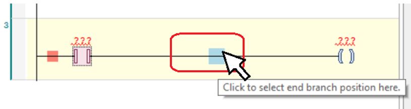
For method 2, to drag and drop the Branch Start/End instruction. Click on Branch Start/End from the toolbox. Grey diamonds will appear on the network suggesting areas to land one end of the branch. Drag to one of the grey diamonds and release.

To complete the second method, notice that now the diamond shapes change to squares. The pink square indicates the start of the branch. Clicking on a grey square will chose where to end the branch. The branch will have doubled vertical lines indicating the branch is capable of something called a Short Circuit Evaluation (SCE). We will discus the SCE in more depth when we learn more about function blocks. It makes little difference if the branch has single or doubled vertical lines for Contacts in parallel.
Whichever method you chose, the result should yield a branch with parallel Contact.

Assign the address for PB4 to the upper Contact. Assign the address for PB5 to the lower Contact and assign the address for the green LED to the Coil.

Once the variables have been assigned, the network is complete. This is a good time to save the project.
To test the network, turn on the simulation mode, login and then start the application.
Write the value TRUE to the upper Contacts and observe the result. Set the upper Contact back to FALSE then write the value TRUE to the lower Contact.

If one of the conditions to the left of the Coil instruction are TRUE, there is a path of logical continuity.
We can summarize, So long as either the upper or lower Contact are TRUE, the Coil is TRUE. The Contacts are for PB4 and PB5. The Coil is for the green LED. This satisfies our program plan, while PB4 or PB5 are pressed the green LED will be on.
The Contact instructions are one below the other on parallel branches, we can say they are in parallel.
Two or more input instructions in parallel have an OR relationship. Any of the instructions with a TRUE condition can provide a path of logical continuity.
Logout and end the simulation.
This concludes Exercise 7. If you did not already save the project this is a good time.
Exercise 8 – Network With Negated Contact
In this exercise we will add to the existing program and create a network that operates with one pushbutton input and one LED output. While we are doing that, we will learn about the Negated Contact and how to reorganize networks by dragging. We will also learn how to add comments.
Do you remember the NOT Operator from the section on Boolean Logic?
For this exercise, our program plan has changed one more time:
- While PB1 is pressed the red LED will be on
- While PB2 and PB3 are pressed the yellow LED will be on.
- While PB4 or PB5 are pressed the green LED will be on.
- While PB1 is not pressed the blue LED will be on.
Step 4 is the new part of the plan and the chosen components are PB1, and the blue LED.

This time, we need to know the addresses for PB1 and the blue LED. Please check the diagram I/O Connections from the section PLC Part 2 Intro To CODESYS. Add the addresses.
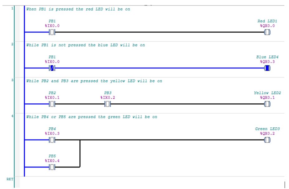
- While PB1 (at address %IX0.0 ) is pressed the red LED (at address %QX0.0 ) will be on.
- While PB2 (at address %IX0.1 ) and PB3 (at address %IX0.2) are pressed the yellow LED (at address %QX0.1 ) will be on.
- While PB4 (at address %IX0.3) or PB5 (at address %IX0.4) are pressed the green LED (at address %QX0.2) will be on.
- While PB1 (at address %IX0.0 ) is not pressed the blue LED (at address ______ ) will be on.
We will add to the existing project. So if the project “Ladder IO Test” is open and the ladder editor for PLC_PRG is open, we are ready to proceed.
From the workspace, we will insert a new network below to create network number 4. Find the Negated Contact instruction and place it, to the left, on the new network. Then place a Coil to the right side of the network.

The Contact and Coil placement should look like this.

Assign the address for PB1 to the Negated Contact. Assign the address for the blue LED to the Coil.

Once the variables have been assigned, the network is complete. This is a good time to save the project.
To test the network, turn on the simulation mode, login and then start the application.
Observe the condition of the network. The condition of the Negated Contact instruction is TRUE. When the value of the address %IX0.0 is FALSE. There is a path of logical continuity.

Write the value TRUE to the Negated Contact. The condition of the Negated Contact instruction is FALSE. When the value of the address %IX0.0 is TRUE. The path is broken.

We can summarize, When the value of the assigned variable is FALSE the condition of the Negated Contact is TRUE. So long as the Negated Contact condition is TRUE the Coil is TRUE. The Contact is for PB1, the Coil is for the blue LED. This satisfies our program plan, while PB1 is not pressed the blue LED will be on.
The condition of a Negated Contact is opposite to the value of the assigned variable.
Logout and end the simulation. Returning to edit mode.
Drag And Drop To Relocate Networks
Network 1 and Network 4 are operated by PB1 at the address %IX0.0. Let’s re-organize the program to keep the networks for PB1 together. Click on network 4 to highlight it as the network being edited. Then click and hold the pink area in the margin. Drag it to the arrow pointing down from network 1 then release.

The network will change position to network 2. Many items in the ladder editor workspace can be moved around in drag and drop fashion.

Commenting
As we keep adding to the program, it becomes more complicated to remember the function of the instructions and networks. Adding comments is a good way to keep organized by documenting how the logic works.
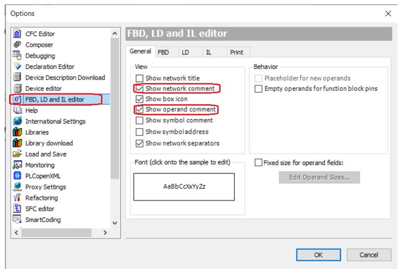
To show comments we must enable the option first. From the Tools menu select Options

Scroll down to FBD, LD and IL editor to adjust editor options. Check the box for Show Network Comment and Show Operand Comment then click OK.
In the workspace, move the mouse pointer to the top of the network area. A grey box will appear. Click on it, the box becomes white and you can type in a network comment.

Type in a comment that describes the purpose of the line of ladder logic.

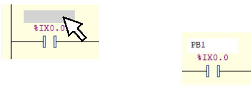
In the workspace, move the mouse pointer to the top of the instruction area. A grey box will appear. Click on it, the box becomes white and you can type in a instruction comment to describe its function.
Go ahead and create comments to document the program.

This concludes Exercise 8. Make sure to save changes to the project
Exercise 9 – I/O Test
This exercise is intended for the PLC training station, as described in the section DIY PLC Training station.

In this exercise, we will connect online with the CODESYS Control Win soft PLC and run the project “Ladder IO Test”. We will exercise every pushbutton and monitor the response from the LEDs. The behavior of the I/O will confirm the correct operation of the training station. We will also learn about forcing I/O.
Here is a list of things to check before we can start:
- The correct project must be open. (in this case “Ladder IO Test”)
- The ladder editor for PLC_PRG should be open.
- The slave device must be connected to the PC with a USB cable. Modbus communications must have been configured as in Exercise 3
- Make sure the CODESYS gateway and soft PLC are running. (See the guide Start Or Stop CODESYS Control Win Soft PLC And Gateway in the Help Section).
- Make sure the Development System is logged off simulation and the simulation mode is off. There should be no red box in the status bar.

Login
Login is required to connect online with the PLC.

When logging in, aside from the usual username and password requirement, the application on the PC is compared to the simulator’s current application, if any. For those reasons you may be prompted by any of the following:
1 . Login credentials. Enter your username and password then proceed. Don’t have a password yet? See the guide Communication Settings Connection Path To PLC in the Help Section.

2 . A dialogue box indicating that no application exists. This happens if the PLC has no application currently loaded Connecting and downloading an application is our objective. So, the correct answer is Yes, to confirm the download.
3 . A dialog box indicating an application is currently loaded but no matching compile information. This happens when the application loaded on the PLC is from different project. Click Yes to confirm the download.

4 . A dialog box with 3 login options. This happens when the application on the PC is does not match the PLC’s current application and you must chose how to proceed.
a) Login with online change – Only loads the changed part of the application and does not require the application to stop to allow the change. This has minimum impact on equipment that may have processes running. Here is an important safety reminder. Making online changes on running equipment can have unpredictable outcomes. Make sure you understand the risks before making online changes on real world equipment.
b) Login with download – Loads the complete application. Any running application would have to be stopped to accept the download. It may automatically restart or a manual restart may be necessary. This has a serious impact on equipment that may have processes running. Here is an important safety reminder. Equipment should be idle and in a Safe Off state if the PLC is being stopped and restarted including for download.
c) Login without any change – No changes will be loaded. The online connection will proceed but the application displayed on the PC will not match what is running on the PLC. This makes the view inaccurate while monitoring from the workspace.
Either of the first two options are acceptable for our purpose. It makes little difference for the training station if we must restart the application. The third option, Login without any change, is not suitable since our objective is to download the application. Once a selection is made then click OK.

5 . A dialogue box indicating no online change is possible. This happens when the application on the PC is significantly different than simulator’s current application. Click Yes to confirm the download.

6 . No connection warning. Check that the soft PLC and gateway are running. See Start Or Stop CODESYS Control Win Soft PLC And Gateway in the Help Section.

7 . No active path defined warning. See the guide Communication Settings Connection Path To PLC in the Help Section.

Once logged in, check the status bar. Is the application running? Click the start button if required. ![]()
Check Modbus Communications
Check for the green, circular arrows in the devices view. They are indicators that the slave device communication is working. Blinking yellow TX and RX LEDs on the board, indicate communication is working as well. Often, when the PLC is first started or after a 2 hour timeout and shutdown, a “bus error” occurs and stops Modbus communication. This can be reset easily, from the Online menu select Reset Warm. After the reset the application will need to be restarted. If communication is not working at this point, see the guide Slave Device Communication Troubleshooting in the Help Section.

I/O Checklist
If communication between the slave device and PLC are working you may proceed to the next step. You can monitor the status of the I/O from the workspace display. Try pressing some of the pushbuttons and watch the blue highlighted regions change in the workspace.
Perform the I/O checklist. Actuate the pushbuttons as described and monitor the response of LEDs.

With any luck it all worked OK, but what if something is not working? What tools do we have to troubleshoot? We can break out most I/O problems into two categories, software and hardware. The software is the PLC application and the hardware would be the slave device. We have tested our program, in simulation mode, as we built each network along the way so that makes hardware the most likely cause.
Sine we can monitor the status of the I/O from the workspace, it is easy to check inputs. For example, to test PB3 we can watch the assigned Contact at address %IX0.2 change status when we push the button. This confirms the electrical operation of the pushbutton, the connection to the Arduino and even the communication of inputs to the PLC.

Forcing
But what about Coils? There is an easy way to test them too. There is something called forcing. For example select the Coil in network 4 at address %Q0.2 and double click. The blue box with the word “TRUE” will appear. Right click anywhere in the workspace and select Force All Values of Device.Application.

The status of the instruction will change, highlighted blue to indicate the Coil condition is TRUE. This should lite up the green LED. If the LED is working this confirms the electrical operation of the LED, the connection to the Arduino and even the communication of outputs from the PLC.

To undo the force, right click anywhere in the workspace and select Unforce All Values of Device.Application. The instruction status will return to normal.

A few more words about forcing. Forcing works on input instructions too. Select any Contact from the workspace and give it a try. Forcing is an easy way to test inputs and outputs but they must be used with care. Not much can go wrong with the training station but on a real machine forcing I/O can have unpredictable results and serious consequences. Here is an important safety reminder. Take care when using forces. Make sure you know what device will be affected and have people stand clear.
Forcing is a great tool but it can cause problems too. Many technicians have wasted time troubleshooting a PLC problem just to find out someone left a force in the program. You can quickly check for active forces by checking the status bar.

Remember, the soft PLC runs for 2 hours intervals, without a license, and then stops. If you see a dialog box declaring No Connection check that the soft PLC is running. Restart if necessary.
During the testing process, if you need to make changes to the application, Logout to edit the logic. Then Login again, confirm the application is running and modbus communication is working. Continue the test.
When you have completed the I/O test. Logout and stop the soft PLC.
This concludes Exercise 9.
Instructions: Set Coil And Reset Coil
Set Coil is an output instruction. It is assigned a variable with BOOL (1 bit) data type. As an output instruction it will control the value of the assigned variable.
The instruction is TRUE if input conditions to the left provide a path of logical continuity. When the instruction is TRUE the bit is set to TRUE ( ON, equals 1) for the assigned variable. The assigned variable will remain TRUE until some other instruction or command acts on it.
The Set Coil can be considered as retentive since it only acts when conditions for the instruction are TRUE, turning the bit ON otherwise the state of the bit is retained.

Reset Coil is an output instruction. It is assigned a variable with BOOL (1 bit) data type. As an output instruction it will control the value of the assigned variable.
The instruction is TRUE if input conditions to the left provide a path of logical continuity. When the instruction is TRUE the bit is set to FALSE ( OFF, equals 0) for the assigned variable. The assigned variable will remain FALSE until some other instruction or command acts on it.
The Reset Coil can be considered as retentive since it only acts when conditions for the instruction are TRUE, turning the bit OFF otherwise the state of the bit is retained.

The Set Coil and Reset Coil instructions are available from the toolbox under the heading Ladder Elements.

Exercise 10 – Light Switch #1
In this exercise we will create a new project and run it with the PLC training station to demonstrate the function of the Set Coil and Reset Coil instructions. We will also explore an old-fashioned seal-in contact arrangement as a comparison.
Our task is this: Given 2 pushbuttons and a light, program ladder logic to turn the light on or off at the entry to the green room. PB1 will be the on button and PB2 will be the off button. The light is the yellow LED, LED2.

Open a copy of the base project “Training_Station_Base” and save as a different project name “Lightswitch”.

Method #1
Before we learned the new retentive output instructions our approach might have looked like an old school seal-in circuit. You may remember the seal-in circuit from Part 1 when we reviewed relay ladder logic.
Open the editor for the program PLC_PRG and place instructions as shown in the diagram titled Seal-In Logic.

Make sure the CODESYS gateway and soft PLC are running. Then Login to connect online with the PLC. Remember how we connected online from Exercise 9.
Check the status bar. Is the application running? Click the start button if required. ![]()
Check for communication to the slave device. Remember how we checked Modbus communications from Exercise 9.
Once the application is running. Monitor the status of the I/O from the workspace display.
Observe, when PB1 is pressed the top line of the network is highlighted blue, the Coil is enabled and the light turns on. The lower branch on the network is highlighted as well. A Contact that monitors the light status and a Negated Contact linked to PB2 provide a second path of continuity.

When PB1 is released, the lower branch keeps the Coil “sealed-in”. The light stays on

When PB2 is pressed, the Negated Contact in the lower branch is no longer TRUE. This breaks continuity to the Coil and the light goes out.

The ladder logic, from method 1, meets the goal to provide working On and Off buttons for a light.
Logout to end the online connection to the PLC and return to edit mode
Method #2
This method utilizes Set Coil and Reset-Coil to accomplish the same outcome. In some circumstances this may be a simpler way.
Start off by deleting the network with the seal-in logic.
(Hint: Clicking on the network will highlight it. Then right click and select delete)
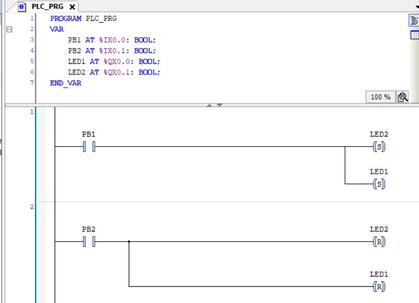
Then create 2 networks.
For network 1, Place a Contact with the address for PB1 and Set Coil with the address for LED2.
For network 2, Place a Contact with the address for PB2 and Reset Coil with the address for LED2.

Make sure the CODESYS gateway and soft PLC are running. Then Login to connect online with the PLC. Remember how we connected online from Exercise 9.
Check the status bar. Is the application running? Click the start button if required. ![]()
Check for communication to the slave device. Remember how we checked Modbus communications from Exercise 9.
Once the application is running. Monitor the status of the I/O from the workspace display.
Note that the Set Coil on network 1 and Reset Coil on network 2 are both the same address. Each network performs a separate action on the output for LED2.
While pressing PB1, observe network 1 highlighted blue. The Set Coil instruction is highlighted blue as well and the light (LED2) is on.

On network 1 when PB1 is released, the network between the Contact and Set Coil is no longer highlighted. But the Set Coil is still highlighted and the LED2 is still on. Note on network 2 the Reset Coil has been highlighted blue ever since PB1 was pressed. It is indicating that the bit for address %QX0.1 is TRUE.

When PB2 is pressed network 2 is highlighted blue up to the Reset Coil. At this point the Reset Coil is no longer highlighted and the light, LED2 is out.

On network 2 when PB2 is released, the network between the Contact and Set Coil is no longer highlighted. The Reset Coil remains unhighlighted.
The ladder logic, from method 2, also meets the goal to provide working On and Off buttons for a light.
Remember to save the project. This concludes Exercise 10
Exercise 11 – Light Switch #2
In this exercise we will add to the project recently created for Exercise 10, “Lightswitch”. The project will be run on the PLC training station. The intention is to demonstrate adding a branch to the right side (output side) of the network and how that splits the signal flow. While we are doing that, we will start learning about declaring variables that are linked to addresses and how that helps keep our logic organized.
Our task is this: Back in the green room, extra lighting has been added to illuminate the stairs. We need to change our logic to control LED1 to operate the same as LED2.

Starting at the workspace. The ladder logic from Exercise 10 is visible.

To add control for the second light we will add Set Coil and Reset Coil instructions, with the address for LED1, to the left side of both networks.
Adding Branches To The Right
To add the output instructions, a branch must be added to the right side of the network to “split-off” the signal. There are 2 ways to do this.
- Placing an additional output instruction on the network This will parallel with the existing output instruction and leaves no room to add other instructions or function blocks to the branch.
- With the Insert Branch instruction. This creates a branch with room to add multiple instructions and function blocks.
For network 1 we will practice the first method, to drag and drop the Set Coil instruction. Click on Set Coil from the toolbox. Grey arrows will appear on the network suggesting to insert the instruction above or below. The arrow pointing to the right will insert below the existing Set Coil and the arrow pointing up will insert above the existing Set Coil. Drag to the arrow pointing to the right and release, creating the branch and the Set Coil below. This is the simplest method for adding parallel output instructions.

For network 2 we will practice the other method. To drag and drop the Branch Insert instruction, click on Branch from the toolbox. Grey diamonds will appear on the network suggesting areas to land one end of the branch. Drag to one of the grey diamonds and release. This creates the new branch. The Reset Coil instruction still must be added.

To complete the second method, place the Reset Coil instruction on the new branch. Its not as simple as the first method but there is room on the branch for more instructions if we were creating more complex logic.

Add the address for LED1 to the new Set Coil and Reset Coil.

Take the usual steps to get logged in to the soft PLC, with the application and slave device running. Once the application is running. Monitor the status of the I/O from the workspace display.
Test the logic. When PB1 is pressed both lights, LED1 and LED2, should turn on. When PB2 is pressed both lights, LED1 and LED2, should turn off.
Once tested, the logic meets the goal to add control for the second light.
Remember to save the project.
About The Branches
The length of the branches is noticeably different. To drive the point home, this is the difference between them:
On network 1 there is room for the Set Coil instruction only. For example if you were to try and place a Contact on the lower branch of network one, there would be no highlighted area or grey diamond suggesting it could land there.
This is not the case for the lower branch on network 2. This type of branch is designed to accept multiple instructions and function blocks to build more complex logic if need be.

Declaring Variables
In a previous exercise, we began using commenting to document the program. Since then we have started fresh with project “Lightswitch” there are few if any comments and no documentation. This is a good time to try something different that can help identify I/O.
Variable names identify a piece of data. A Declared Variable is a variable created by the programmer by giving a name and a data type. We can use variable names to identify I/O. Warning: When declaring variables keep in mind that variable names cannot have spaces. If you are using a multiword name, use an underscore instead of a space.
Logout to end the online connection to the PLC and return to edit mode. In the workspace at network 1, click on the address %IX0.0 and type in “PB1” then press enter.

A dialog box titled Auto Declare will appear. The field for Scope is VAR, which is a normal variable. The Object Field will show PLC_PRG[Application] indicating that the variable is valid within the POU named PLC_PRG for the current application.
The variable name and type are already present. You need to type in the address for PB1, %IX0.0. This will link the address to the variable. Then click OK.

Note: If the Auto Declare box does not appear automatically, you can prompt it by selecting the desired text and pressing the Shift and F2 buttons at the same time.
The assigned variable for the Contact on network 1 is now PB1. To the top of the workspace is the declaration editor. It shows the local variables defined for the program PLC_PRG. In the declaration editor we see a new line “PB1 AT %IX0.0: BOOL;”. This shows the declaration we have just made. It includes the variable name and data type. It also contains the AT code to link a specific address. This is how we linked the variable to the pushbutton PB1.

Using the Auto Declare Box, go ahead and declare variables for PB2, LED1 and LED2, make sure you link to the correct address. Once a variable name has been declared it is available to use for multiple instructions within the POU. Note that LED1 and LED2 are declared once but appear in two different places in the logic. Remember variable names cannot have spaces.
Back to the situation in the green room.
If someone enters the area from upstairs, access to the light control is required. How can we add PB3 and PB4 to the program to control the lights from upstairs as well? With what you have learned so far try to create your own solution and then test it.

(Hint: A solution is provided at the beginning of Exercise 12. You can compare your work to what is shown there but give it a try before you look ahead.)
Make the changes to the program. Login to connect online with the PLC and test the program. When you are satisfied, logout and stop the PLC. Remember to save the project.
This concludes Exercise 11
Quick Change Commands, Set/Reset And Negation
A feature of the editor that should be mentioned, is the capability to quickly change the type of Contact or Coil using the Set/Reset and Negation commands.
The commands are easily available in 3 places:
1 . From the toolbar.

2 . Select from the FBD/LD/IL dropdown menu.

3 . Right click on the element being edited, a menu will appear with a list of instructions.

The Set/Reset command will toggle a selected Coil between 3 states: Set Coil, Reset Coil and Coil. If you highlight the Coil and apply the command the instruction will change.

The Negation command will toggle a selected Contact between 2 states: Negated Contact and Contact. If you highlight the Contact and apply the command the instruction will change.

It may be used less frequently, but the Negation command can be applied to other elements as well:
On network segments and block inputs/outputs it will appear as around dot called a Negation Symbol. Whatever the logic condition may be to the left of the symbol, it will be opposite to the right.

When the Negation command is applied to Coils, they become Negated Coils. The output of a Negated Coils is the exact opposite of what a Coil would have been.

Another quick way to change instructions is to drag and drop the desired item from the toolbox into place. For example, to change a Contact to a Negated Contact, click and hold Negated Contact from the toolbox and drag to the network area. A grey square will appear with the letter “R”. R stands for Replace. Bring the mouse cursor to the square until it turns green then release to replace the instruction.

This method works to swap out Coil, Set Coil and Reset Coil instructions as well.
Thank you for reading the learning series, PLC Part 3 Basic Ladder Diagram.
Click on this link to proceed to the next section PLC Part 4 Timers Counters & Triggers.
References – Books And Weblinks
You can explore more on the subjects discussed in PLC Part 3 Basic Ladder Diagram with these links.
CODESYS – Codesys help website – https://help.codesys.com/
Arduino Uno – Arduno Learn website – https://docs.arduino.cc/learn/
Open PLC and Slave Device – Open PLC Project website – https://www.openplcproject.com/